William C. Hall

UALR Department of Physics

REU-FOM/SILL

 

 

The existence of extended states in quantum Hall type systems

 

 

Introduction

 

Studying extended states is important to physicists trying to understand the transport properties of various materials, because the extended states play an important role in determining these transport properties. Generally, if the relative abundance of extended states in a system is high, then the material in which the system exists will allow current or heat to flow through it very well. Extended states are ones in which the electrons have a relatively large probability of appearing across a large portion of a macroscopic sample. This is the exact opposite of localized states, which have a large probability of existing in a relatively small portion of a macroscopic sample.

In particular, we are interested in single electron states in a 2-dimensional (2D) electron system, meaning the electrons are confined to move only parallel to the surface of a sample material and not perpendicular to it. For example, a 2D electron system can be “realized at the surface of a semiconductor like silicon and or gallium arsenide where the surface is usually in contact with a material which acts as an insulator ( for silicon field effect transistors and, e.g.  for heterostructures). Electrons are confined close the surface of the semiconductor by an electrostatic field  normal (pointing downward) to the interface, originating from positive charges which cause a drop in the electric potential toward the surface” (K. von Klitzing). In this 2D system, there is an electrical interaction that varies across the surface, the “impurity” potential, whose physical origin varies. For example, in the integer quantum Hall effect it is due to atoms being substituted or displaced, whereas in the fractional quantum Hall effect it is due to the other electrons. In addition, there is a uniform magnetic field that is perpendicular to the plane of the surface. Our goal is to understand, using computer simulations, the number and energy dependence of extended states for electrons constrained to 2D motion in the presence of a strong magnetic field perpendicular to the plane of motion and this impurity potential.

We use the root-mean-square radius ( ) and participation function (P) to quantify the extension of eigenstates in these systems.   is a measure of the average radius of a state, while P is a measure of an area. We first analyze  and P as functions of eigenenergies for the single electron states. If either  or P is equivalent to the size of the system, then we know that state is extended. We also graph and analyze the ratio , from which we can determine whether the states are disk-like (relatively large area and radius) or ring-like (relatively large radius and a small area). Finally, we will analyze the extended states and energy dependence of  and P as a function of the distribution of the impurities, their shape, and their number relative to the strength of the magnetic field.

 

 

Methods

We study extended states by using two measures of extension: root-mean-square radius  and the participation number (P). Roughly speaking,  measures the radius of an eigenstate, while P measures its area (Horner, pg 17). We chose to use  and P because they do not measure the same things, and they are both arguably relevant to extension: a large radius crosses the system while a large area covers the system.  is given by , where  is the expectation of the operator , and is equal to . P is given by . In both cases,  is the wave function of a single electron.  gives the normalized probability of a wave function. For our methods, we can express  in terms of  and . We will look at two simple cases, which will give us a better idea of what  and P mean. We can first find  for a disk. The idea is that we want a disk where the probability is constant inside the disk and zero outside the disk and we require that if we integrate the probability density over all space we will get 1. We want our single electron to exist in the disk, but nowhere else. Thus, we have that

  , where C is the normalization constant and  is the area of the disk. Since C, then  (disk) . We can now do the same steps for a thin ring, except we integrate  from 0 to , and  from  to , where  is the thickness of the ring. Thus have that  (thin ring). Now that we have calculated the values of  for a disk and a thin ring, we can find  and P for a both a disk and a thin ring. Thus, we have that

 (disk)

P (disk)

(thin ring)

P (thin ring)

Comparatively speaking, a ring-like state at the edge of a system would show a large radius but not a large area because of its thinness, while a disk-like state would show a large radius and a large area as well. Both    and P show larger values for extended states than for localized states.

         Once we have calculated the and P of the states, we graph the results of  and , which are scaled to system size, as a function of their eigenenergies. We scale to system size because it makes it easier to compare results for different system radii. We use  instead of P since we want to compare lengths instead of areas in our analyses. We know that if the highest peak value of  goes to 1, then the radius of the state is the same as the radius of the system and there is definitely an extended state. When we look at the peak of , a value of approximately 1.77    would indicate there is an extended state. We then graph the ratio , which is a measure of the degree to which a state looks like a disk or a ring (Horner, L. pg 19). In the near future, we will analyze the impurities of  and  as a function of the number of impurities relative to the strength of the magnetic field, the shape of the impurities, and the distribution of the impurities.

 

Results

         In my particular case, I am studying single electron states in 2D electron systems where there is only one impurity. The following three graphs (figures 1, 2, and 3) are a sample of some of the results that I obtained for this type of system.

Figure (1) is a graph of the  (scaled to system size) as a function of eigenenergy. Of particular interest to us is the peak on the left side of the graph. It represents the most de-localized state, which is crossing most of the system. Notice that the peak value is 1. This means, as we explained earlier, that there is an extended state since the radius of the state extends across the radius of the system . Other examples are less clear as to whether there are extended states, since their peak values are large but not 1.

          

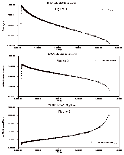
         Figure (2) is a graph of the  as a function of energy.  is scaled to system size as well. The same thing is happening here as in figure 1, only now the peak value measured (slightly higher that 0.75) is less than the value of 1.77 needed for extension. We can now say that there are not any disk-like states that cover the whole system in this particular system.

         Figure (3) is a graph of the ratio . It is not completely clear to us at the present time if this graph will prove directly useful to us in our current work. However, it does show us that the  and  are different ways of measuring the extension of a state, since the graph is not a straight line. This graph helps us to understand what is meant by extended states by implying that if you look at extended states at some level, you have to be more specific about how you define extended states, since you now have a choice in what you want to call extended.

         In the future, after accumulating enough data from many different small system sizes, and extrapolating to an infinitely large system, we will graph and analyze the  and  as  functions of the number of impurities relative to the strength of the magnetic field, the distribution of the impurities, and their shape. We want to know if the results we get will be any different from those obtained when we graphed the and  as functions of their energies for this system.

 

Summary

         We are interested in the existence and energy dependence of extended states in quantum Hall type systems. We have computed the root-mean-square radius ( ) and participation number (P) as a function of energy   for a few system sizes. Our next step is to analyze the peak values of  and P as a function of “impurity” distribution, shape, and number relative to the strength of the magnetic field.  

 

BIBLIOGRAPHY

 

Aoki, H., Computer simulation of two-dimensional disordered electron systems in strong magnetic fields, J. Phys. C: Solid State Phys., vol. 10 (1977) pp. 2583-2593.

 

Gedik, Z. and M. Bayindir, Disorder and localization in the lowest Landau level in the presence of dilute point scatterers, Solid State Communications vol. 112 (1999) pp. 157-160.

 

Horner, M.L., Transmutation of Electric into Magnetic Forces on a Planar Electron: Impurity Spacing and Band Structure in Strong Magnetic Fields, Disssertation (1999), State University of New York at Stony Brook

 

Jain, J. K., The Composite Fermion: A Quantum particle and its quantum Fluids, Physics Today, vol. 53 no. 4 (April 2000) pp. 39-45.

 

von Klitzing, K., The quantized Hall effect, Nobel Lecture (1985), Max-Planck-Institut für Festkörperforschung, D-7000 Stuttgart 80.

 

Störmer, H.L., D.C. Tsui and A.S. Gossard, The fractional Hall effect, Reviews of Modern Physics, vol. 71 no. 2 (1999) pp. S298-S305.

 

Thouless, D.J., Electrons in disordered systems and the theory of Localization, Physics Reports, vol. 13 no. 3 (1974) pp. 93-142.