A very fast intro to decision theory

There are 4 basic elements in decision theory: acts, events, outcomes, and payoffs. Acts are the actions being considered by the agent -in the example elow, taking the raincoat or not; events are occurrences taking place outside the control of the agent (rain or lack thereof); outcomes are the result of the occurrence (or lack of it) of acts and events (staying dry or not; being burdened by the raincoat or not); payoffs are the values the decision maker is placing on the occurrences (for example, how much being free of the nuisance of carrying an raincoat is worth to one). Payoffs can be positive (staying dry) or negative (the raincoat nuisance). It is often useful to represent a decision problem by a tree.

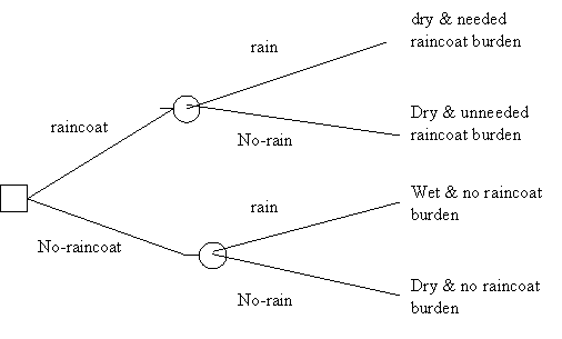
Here a square indicates a node in the tree where a decision is made and a circle where events take place. The tree does not contain payoffs yet, but they can easily be placed by the outcomes.

In general, we can note two things. First, the nature of the payoffs depends on one’s objectives. If one is interested only in making money, then payoffs are best accounted for in terms of money. However, if one is interested in, say, safety, then the payoffs are best accounted for in terms of risk of accident, for example. If any numerical approach is possible when disparate objectives are involved, there must be some universal measurable quantity making them comparable. (In fact, utility, of which more later, is such a quantity). Second, decision making trees can become unmanageable very fast if one tries to account for too many possibilities. For example, it would be physically impossible to account for all the possibilities involved in the decision of which 50 out of 200 gadgets should be intensively marketed, as the number of possible combinations, 200!/(50! ∙ 150!) is simply astronomical. Hence one must use good judgment in limiting the options considered; this is potentially problematic, as one may unwittingly fail to consider a possible action which would produce very good outcomes.

Decision Criteria

How one uses a decision tree or a decision matrix depends on the decision criteria one adopts. Consider the following payoff matrix where acts are rows, events columns, and the resulting squares contain the payoffs (outcomes are not represented to avoid clutter). So, suppose that we are considering which widget out of 3 to produce and our goal is making money.

	EVENTS
	Good sales	Bad sales
ACTS
Produce A	+$5000	-$1000
Produce B	+$10000	-$3000
Produce C	+$3000	-$500

Here producing B is obviously the best option if things go well, while producing C is the best option if things go badly, as losing $500 is the best of the worst payoffs. The decision criterion telling us to choose C is called “Maximin”. Obviously maximin is a rather pessimistic strategy, and for this reason it is controversial. However, if the stakes are very high (for example, suppose that if I lose more than $500 I will be forever ruined), maximin seems a reasonable option. The application of maximin in the original position has played an important role in Rawls’ A Theory of Justice, the most important work in political philosophy in the last decades. Other decision criteria in cases of uncertainty are maximax, minimax of regret, and the appeal to subjective probabilities through the Principle of Indifference. Unfortunately, none of these principles is always viable.

However, when the probabilities of events are available (that is, in decision under risk) and the agent is indifferent to risk, as when the payoffs involved are significant but not too significant, the criterion usually put forth in decision theory is that of the expected maximum payoff (EMP), the counterpart of the principle in gambling enjoining us to choose the bet with the greatest expected value. So, suppose that we could provide the relevant probabilities, as in the following matrix:

	EVENTS
	Good sales	Bad sales	Payoff	Expected payoff
ACTS
Produce A Pr(good sales)= 80% Pr(bad sales) =20%	+$5000 x 80% = 4000	-$1000 x 20% = -200	+$4000	+$3800
Produce B Pr(good sales)= 60% Pr(bad sales) =40%	+$10000 x 60% = 6000	-$3000 x 40% = -1200	+$7000	+$4800
Produce C Pr(good sales)= 50% Pr(bad sales) =50%	+$3000 x 50% = $1500	-$500 x 50% = -$250	+$2500	+$1250

Then, EMP would tell us to produce B, as the expected payoff is the greatest. Most business decisions fall into this category. For example, if a company makes dozens of decisions with comparable payoffs every day, then EMP is the best business strategy, as it is for a casino.

Decision trees and backward induction

Typically, more than one decision is involved in decision making, in which case it is best to use a tree instead of a matrix. For example, consider the following situation, in which no probabilities are involved.

You have arrived at a fork in the road on you way home.

If you go left, you’ll have to go through a very sunny patch in the mid of a very hot day. However, this will also allow you to admire a beautiful bloom of wildflowers growing by the side of the path. You shall then arrive at another fork. If you take another left, you will have to go by a neighbor’s house with a very unpleasant guard dog that will growl at you from the other side of the fence. By contrast, if you go right at the second fork, you’ll go by a very noisy and dusty part of the road. Whichever of the two you take, you shall get home quickly.

If you go right at the first fork, you’ll go through the woods, which are very cool this time of the year. However, there will be little to admire until you get to another fork in the road. If you go left at this fork, you will see some beautiful meadows; unfortunately, it will take you longer to reach your home, a bad thing since you are in a bit of a hurry. If you go right, you shall get home in good time.

Suppose that you assign the following utilities:

Getting hot: -10; seeing the wildflowers: +15; being growled at: -3; pleasant coolness: +10; being a bit late getting home: -5; taking a noisy and dusty road: -2; seeing the nice meadows: +4; getting home in good time: +2.

We can construct a decision tree.

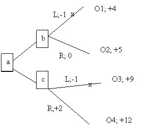
Decision trees can be used by applying backwards induction. The idea is that in order to determine what to do at a (the decision at the first fork), one needs to decide what one would do at b and c. In other words, the tree is analyzed form the right (from the outcomes) to the left (to the earlier decisions). So, at b, one would take the right path because it leads to outcome O2 with utility is +5 while the utility of the left path leading to O1 is +4. We can represent this choice by pruning the left path, that is, by placing an ‘x’ on it. By the same token, at c one would choose to go right, and therefore we may place an ‘x’ over the left option. We are now left with a simplified tree at a: going left will have utility +5, while going right will have utility +12. Hence, we should go right twice.

Adding probabilities

The previous example did not involve probabilities. However, introducing them is not much of a problem, as the following example shows.

You are about to produce a new garment C and must determine whether to merchandise it only nationally (N) or internationally as well (I).

If you choose N and sales are good (G), then you’ll make 4, and if they are bad (B) you’ll lose 1. (All payoffs are in millions). You believe that the probability of good national sales is .8 and that of bad national sales is .2. You must also decide whether to produce and sell a matching scarf S. If S’s sales are good, you’ll make an additional 2, and if they are bad you’ll lose an additional 1. You think that if C sells well the probability that S’s sales are good is .9 and the probability that S sells badly is .1. By contrast, if C sells badly, the probability that S’s sales are good is .4 and the probability that S sells badly is .6.

If you choose I and sales are good you’ll make 6, and if they are bad you’ll lose 2. You believe that the probability of good sales is .7 and that of bad salses is .3. As in the other case, you must decide about S. If S’s sales are good, you’ll make an additional 3, and if they are bad you’ll lose an additional 2. You think that if C sells well the probability that S’s sales are good is .8 and the probability that S sells badly is .2. By contrast, if C sells badly, the probability that S’s sales are good is .4 and the probability that S sells badly is .6.

Because of the seasonal nature of your business, you need to decide now, a few months in advance, what to do.

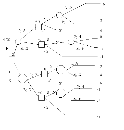
The tree below digrams the decision. Obviously, the first decision is whether to choose N or I. Let’s follow the subtree tree arising from N, as that stemming from I is analogous. Upon deciding N, there is an act of nature, hence the circle with G (good sales) and B (bad sales). After G, we write .8, which is the probability of good sales if you choose N. Your second decision regards S, which is represented by the square with the two branches S (produce and sell S) and ~S (don’t produce S). If you choose S, then the sales can be good or bad (an act of nature) represented by the circle and the relevant probabilities; if you choose ~S, then you are left with the gains or losses from selling C nationally. The payoff are easy to calculate. Conside the uppermost branch, representing your choice of N, good sales of C, your choice of S and good sales of S. Since C sells well, you make 4 and since S sells well, you make 2, so that the total payoff for this branch is 4 + 2 = 6. The second topmost branch has a payoff of 3 because although C sells well (you gain 4), S does not (you lose 1).

The tree is analyzed by backward induction. Starting at the top, the last decision you make is whether to choose S or ~S. The expected payoff of choosing S is 5.7, which is 6 times .9 plus 3 times .1, exactly as if we were considering a bet in which you get 6 with probability .9 and 3 with probability .1. Since 5.7 > 4, you clip ~S, which simply means that the best decision given N and good sales of C is to choose S. Since 5.7 is the best expected payoff available, we write 5.7 next to the relevant square. By contrast, given N and bad sales of C, the best option is ~S, with payoff of -1, as the option S has an expected payoff of -1.2. Hence, S is clipped. We can now calculate the expected payoff of choosing N, namely 5.7 times .8 plus -1 times .2, which is 4.36. We write this figure next to the choice N. The lower half of the tree is analyzed analogously, resulting in an expectd payoff of 5 for I. Since 5 > 4.36, N is clipped and I is the best choice, that with the highest expected payoff.

Revising decision trees in the light of new information

Consider the following scenario. You have to choose which of two widgets, A and B, to market. You also believe that the probability of high demand for A is 80% and the probability of high demand for B is 30%. (High and low demands are the only two alternatives). However, while you get only $3 for every sold A, you get $5 for every sold B. Suppose that if an item is in high demand you shall sell 10,000 of them and with low demand only 4000. Item A cost $1 to produce, while item B costs $2. Moreover, time constraints due to the holiday season compel you to produce 10,000 items of whichever of the two widgets you decide to market. What should you do?

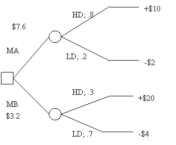
We already know how to construct the decision tree listing the outcomes and the payoffs in thousands. For example, since 10,000 items must be produced no matter what the sales will be, the production cost of A is 10. If A sells well, all 10,000 will be sold, with a gain of 20. Hence, the payoff will be 20-10=10. If demand is low, only 4,000 will be sold, with a gain of 8. Hence, the payoff will be 8-10=-2.

By regressive induction, we see that MA has an expected payoff of 7.6 and MB of 3.2, which means that we should choose MA.

Suppose, however, that you submit A and B to a buyer panel; the reliability of the panel is given by the following figures: in the past, out of 100 high demand items, the panel was positive (P) about 70 and negative (N) about 30; out of 100 low demand items, the panel was positive about 20 and negative about 80. (Note that high or low demand is built into the market, and therefore is the conditioning factor in conditional probability). In short,

Pr(P|HD)=70%; Pr(N|HD)=30%; Pr(N|LD)=80%; Pr(P|LD)=20%.

To make use of this new information, we use Bayes’ theorem to determine the posterior probabilities of HD and LD, that is, their probabilities given the panel’s results. The relevant probability, not decision, tree is

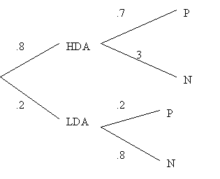
Hence, by Bayes’ theorem (with figures adjusted to 2 decimals):

Pr(HDA|P) = .93; Pr(LDA|P) = .07

Pr(HDA|N) = .6; Pr(LDA|N) = .4.

By an analogous procedure, one obtains

Pr(HDB|P) = .6; Pr(LDB|P) = .4

Pr(HDB|N) = .14; Pr(LDB|N) = .86.

At this point we can rewrite the decision tree incorporating the new posterior probabilities:

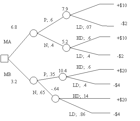
From now on it is just a matter of employing backward induction to determine which widget to market. The expected payoff of marketing A if the panel has a positive reaction is +$7.9; if the panel has a negative reaction the expected payoff drops to +$5.2. With respect to B, if the panel has a positive reaction, the expected payoff is $10.4; if the panel has a negative reaction, it becomes -$.64. The expected value of marketing A is 6.8; that of marketing B is 3.2. Hence, one should market A. Since the expected payoff difference between MA and MB is 3.6, one should pay less than 3.6 for the panel; in other words, given the data of the problem, the extra information is not worth more than 3.6.

One can easily see that decision trees could get complex and difficult to construct. For example, getting the information may take time when time is of the essence (perhaps, A and B are holiday season widgets). Moreover, in our examples we came up with the relevant probabilities by fiat. In real situations, of course, coming up with the correct probabilities can be very difficult, especially when appealing to history or statistical surveys does not help. However, such cases are best left to a decision theory course.