Ternary Plots
Up to now, we have considered the frequency of strategies in games involving only two strategies. We now consider a particularly interesting case of a game with three strategies, Rock-Paper-Scissors. However, before we do that we need to look at ternary plots, a common way to represent the phase space of such games.

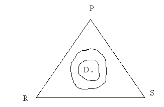
Consider the equilateral triangle RSP and the segments DA, DB, and DC, which are the distances of D from side RS, SP, and PR, respectively. Vertex R represents the strategy Rock, vertex S Scissors and vertex P Paper. Any point D in the triangle, icluding the interior area, sides, and vertices, represents a probability distribution of the strategies, with distance DA representing the frequency of Paper, DB that of Rock, and DC that of Scissors. Note that any two of such distances fully determines the strategy distribution. The distance between a vertex and the opposite side is normalized, which means that when the point D concides with a vertex, that vertex’s strategy is the only left. For example, when D concides with P, the frequency of P is 1. By the same token, if D is located on a side, then the frequency of the strategy of the opposing vertex is zero. For example, if D is located on RS, then the frequency of P is zero.
Rock-Paper-Scissor
Rock-Paper-Scissor is a game in which Rock (R) beats Scissors (S), Scissors beats Paper (P) and Paper beats Rock, so that the relation ‘X beats Y’ is not transitive. Mathematically, the game is easier to handle if
· the strategy order in the matrix is R, S, P
· the payoffs on the main diagonal are 0. (Remember one can always obtain this by subtracting the same quantity from every box in the same column).
Hence, we
assume that these two conditions are satisfied, otherwise the procedures below
will not work.
|
|
R |
S |
P |
|
R |
0 |
1 |
-1 |
|
S |
-1 |
0 |
1 |
|
P |
1 |
-1 |
0 |
Table 1
In the matrix, 1 represents winning, -1 losing, and 0 a tie. Assuming that winning and losing represent invasion rates of one species or one morph against another, the generalized matrix for the game is
|
|
R |
S |
P |
|
R |
0 |
a |
-b |
|
S |
-c |
0 |
d |
|
P |
e |
-f |
0 |
Table 2
where the invasion rate is between and including 0 and 1, with 1 representing the case in which the winning strategy completely replaces the defeated one. Note that when a=c, b=e, and d=f the game is zero sum, and when a=b=c=d=e=f=1 we are back in the classic RPS game.
In replicator dynamics, the following is true:
- There is only one internal fixed point (an equilibrium point), which is associated with the mixed strategy Nash equilibrium.
- If p is the frequency of P, r that of R and s that of S at the internal fixed point, then the following holds:
p=αa, r=αd, s=αe,
with α = (a+d+e)-1, which is the inverse of the sum of the invasion rates.
- If the determinant Δ of the payoff matrix is less than zero (Δ < 0), then the interior fixed point is an unstable center, with trajectories spiraling out asymptotically to the sides. (In computer simulations eventually one strategy vanishes by rounding, and one of the remainig two takes over). In the RPS matrix, Δ = ade - bcf.

- If the determinant Δ = 0, then the interior fixed point is a center of stable orbits circling around it.
- If the determinant Δ > 0, then the interior fixed point is globally stable, with the orbits exhibiting damped oscillations convergint to it.

(1)-(2) entail that the frequency of a strategy at the interior equilibrium is not determined by its own invasion rate but by that of the strategy it invades. For example, the frequency of P is proportional to a, the invasion rate of R. Consequently, if a strategy has the highest invasion rate, then its invader has the highest frequency at equilibrium, and if it has the lowest invasion rate, then its invader has the lowest frequency.
In finite population simulations:
- The orbits spiral out towards the sides
- The species with the lowest frequency at the interior equilibrium has the lowest frequency along every orbit, and consequently the greatest probability of extinction.
Hence, strategy X with the lowest invasion rate is the one most likely to survive, as its invader will vanish, with the result that X will displace that remaning strategy. In short, the game results in the survival of the weakest, as it were. In practice, if strategies are replaced by species or morphs, and a disease, or human intervention, weakens one of them by diminishing its invasion rate, then that species or morph is the most likely to survive.
As an example of RPS, consider the following matrix, where payoffs are invasion rates:
|
|
R |
S |
P |
|
R |
0 |
.2 |
-.4 |
|
S |
-.5 |
0 |
.8 |
|
P |
.3 |
-.6 |
0 |
Then, α = 10/13, so that r = 8/13, s = 3/13, and p = 2/13. Note that r+s+p=1, as normalization requires. As the determinant Δ = (48/1000 - 120/1000) < 0, it follows that under replicator dynamics the interior equilibrium is unstable.
If the population is finite, then P will eventually disappear, thus leaving R as the sole survivor. Note that R has the lowest invasion rate.
Many species or morphs from unicellular organisms to
vertebrates, can be studied using RPS, including E. Coli (a microbe in our guts), Uta Stansburiana (a