Probability Density and Quantum Mechanics
4.2 Schrödinger’s Wave Function
Consider a
particle moving along the x-axis. Quantum mechanics determines the probability of observing the particle in
a given position at a given time by using the wave function ![]() of the particle. One gets
of the particle. One gets ![]() by solving the Time
Dependent Schrödinger Equation (TDSE),
by solving the Time
Dependent Schrödinger Equation (TDSE),
![]() (4.2.1)
(4.2.1)
where V is the (classical) potential energy determined by the physical
system under investigation, m the
mass of the particle, and ![]() (h-bar) is Plank’s
constant. [1] In other words, the wave function is a
solution of TDSE. Setting up TDSE and
solving it can be (and often is) difficult.
However, all we need to know is that the relationship between the wave
function, probability, and physical reality is given by Born’s statistical interpretation:
(h-bar) is Plank’s
constant. [1] In other words, the wave function is a
solution of TDSE. Setting up TDSE and
solving it can be (and often is) difficult.
However, all we need to know is that the relationship between the wave
function, probability, and physical reality is given by Born’s statistical interpretation:![]() , the normalized squared modulus (the square of the
absolute value) of the wave function, is the probability density that upon
observation the particle will be found at point x at time t. For
example, suppose that at time
, the normalized squared modulus (the square of the
absolute value) of the wave function, is the probability density that upon
observation the particle will be found at point x at time t. For
example, suppose that at time ![]() ,
, ![]() is the curve in figure
4.
is the curve in figure
4.
Figure 4
Then, the area under ![]() between a
and b is the probability that a
position measurement at time t1 will return a value between a and b. The key word here is
“measurement”. That is, at least in the
minimalist version we consider, quantum mechanics makes predictions only about
measurement returns. In other words, all
it tells us is what returns we shall have, and with what probability, if we
perform such and such an experiment, without making any claims about quantum
particles outside of the experimental setting.
between a
and b is the probability that a
position measurement at time t1 will return a value between a and b. The key word here is
“measurement”. That is, at least in the
minimalist version we consider, quantum mechanics makes predictions only about
measurement returns. In other words, all
it tells us is what returns we shall have, and with what probability, if we
perform such and such an experiment, without making any claims about quantum
particles outside of the experimental setting.
4.3 The Harmonic Oscillator
Consider a cube on
a frictionless plane attached to a spring fixed to a wall. Suppose that the system is in an equilibrium
position, corresponding to the relaxed length of the spring so that the box is
at rest (Fig. 5). Let us take the origin
0 of the x-coordinate to be the position where the center of box is. Now, we stretch the spring to the right so
that the center of the box is at ![]() and then we let
go. Obviously, the box will be pulled
back by the spring, acquire energy which will be spent compressing the spring
until its center reaches
and then we let
go. Obviously, the box will be pulled
back by the spring, acquire energy which will be spent compressing the spring
until its center reaches ![]() . Then, it will be
pushed again by the compressed spring to the position it had when we let the
box go. In short, in the absence of
friction or external forces the box will forever oscillate back and forth
between x1 and x2 with simple harmonic
motion. Such a system is a harmonic
oscillator.
. Then, it will be
pushed again by the compressed spring to the position it had when we let the
box go. In short, in the absence of
friction or external forces the box will forever oscillate back and forth
between x1 and x2 with simple harmonic
motion. Such a system is a harmonic
oscillator.
Figure 5
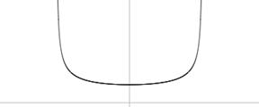
The probability density for the classical harmonic oscillator is plotted below (Fig. 6).
![]()
![]()
![]()
![]()
![]()
![]()
![]()
![]()
Figure 6
x1 and x2 are called “turning points” because the center of the box cannot go beyond them: doing so would be contrary to the laws of classical (Newtonian) mechanics. The plot tells us that if we take random snapshots of the box, the bulk of the snapshots will depict the box near the turning points. On reflection, this is how we would intuitively think it should be, since the box moves the slowest close to the turning points and the fastest close to point 0 in the middle of the run.
However, when we consider the
quantum harmonic oscillator, we are in for some big surprises. First we need to plug the (classical)
potential energy formula ![]() (where k is a constant measuring the
springiness of the spring and x is
the spring’s displacement) for the harmonic oscillator into TDSE. Once we have solved TDSE and obtained the
wave function, we need to normalize its square modulus. Although this is too complex for us to
tackle, amazingly it turns out that the
mathematics of normalization forces the quantization
of energy. While the classical harmonic
oscillator can have any energy level (between any two energy levels, one can
always find a third), the quantum harmonic oscillator can only be found to have
discrete and very definite energy levels E0,
E1, E2,…. In
addition, while in the classical case the lowest energy level is zero
(corresponding to the state in which the spring is relaxed and the box does not
move), in the quantum case the measurement return for lowest possible energy
(the energy of what is called “the ground state”) is
(where k is a constant measuring the
springiness of the spring and x is
the spring’s displacement) for the harmonic oscillator into TDSE. Once we have solved TDSE and obtained the
wave function, we need to normalize its square modulus. Although this is too complex for us to
tackle, amazingly it turns out that the
mathematics of normalization forces the quantization
of energy. While the classical harmonic
oscillator can have any energy level (between any two energy levels, one can
always find a third), the quantum harmonic oscillator can only be found to have
discrete and very definite energy levels E0,
E1, E2,…. In
addition, while in the classical case the lowest energy level is zero
(corresponding to the state in which the spring is relaxed and the box does not
move), in the quantum case the measurement return for lowest possible energy
(the energy of what is called “the ground state”) is
![]() , (4.3.1)
, (4.3.1)
a quantity greater than zero, albeit a very small one.[2] The measurement returns of all the other possible energy levels (the energies of the excited states) are multiples of E0 according to the formula
![]() . (4.3.2) When it comes to
position measurements, things are as strange, as we can gather from figure 7,
which provides the plots of the probability densities for the first four energy
levels. (The intersection points between
each probability density and the parabola at an energy level are the classical
turning points for that energy level).
. (4.3.2) When it comes to
position measurements, things are as strange, as we can gather from figure 7,
which provides the plots of the probability densities for the first four energy
levels. (The intersection points between
each probability density and the parabola at an energy level are the classical
turning points for that energy level).
x E0 E1 E2 |Y(x)|2
![]()
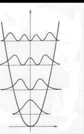
Figure 7
In an excited state En, there are n positions in the space between the turning points where the particle will never be found. In particular, in all odd states such as E1 or E3 the probability of finding the particle exactly in-between the turning points is zero. In addition, the probability of finding the particle outside the classically permitted range (beyond the turning points) is not zero, a phenomenon called “tunneling”. In fact, it turns out that the lower the energy, the greater the probability that the particle will tunnel: at the ground level, the probability of tunneling is slightly above 15%. Tunneling is a pervasive phenomenon at the quantum level: it allows the sun to burn (and life on earth to exist) and matter to escape from black holes.