1. Introduction

Economic geographers in recent decades have been paying more attention to trade as a new way of conceptualizing spatial economic relations. However, there have been several shortcomings in their study of trade mechanisms. One is the near total confinement to the two-country and two-commodity model, neglecting the more general multi-country and multi-commodity framework. Another problem is that most of the existing trade models are not flexible enough to reflect relationships between different trade theories. In addition, there has been scant attention given to the relationships between trade theory and location theory, the latter of which was the major conceptual basis of economic geography prior to the 1970s. This paper addresses these shortcomings. The second section will develop a trade model capable of addressing the first two problems. The third section recasts location theory in an exchange framework by applying the trade model developed in the first section to central place theory, agricultural/land use theory, and industrial location theory.
 

2. Absolute advantage, comparative advantage, increasing returns to scale, and competitive advantage

Any discussion of trade and exchange will involve the original conceptual twins, absolute advantage by Smith (1776) and comparative advantage by Ricardo (1817). The absolute advantage principle attributes trade to differences in productivity. A commodity using less input in production is said to have absolute advantage and should be exported. In essence, Smith uses the number of hours used in making a unit of commodity as the measure of value and thus a unit of account (or the numeraire) in exchange. Classical comparative advantage promulgated by Ricardo identifies an alternative reason for trade; the comparative advantage, which measures the cost of one commodity in terms of another. A commodity that requires sacrificing less of the second commodity is said to have lower comparative cost and should be exported. Essentially, Ricardo introduces a commodity, instead of labor hours, as the numeraire in exchange.

Initial model.

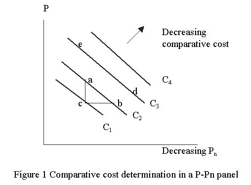
To discuss trade mechanism, a simple model is developed. Denote the productivity of a commodity as P and productivity of the numeraire commodity as P_n. The comparative cost of the commodity measured in the numeraire is C=P_n/P. In the P-P_n panel shown in Figure 1, the vertical axis expresses P and the horizontal axis expresses decreasing P_n. A given level of C can be obtained with different combinations of P and P_n. For example, increasing (decreasing) P_n accompanied by proportionately increasing (decreasing) P leads to a downward-sloped iso-cost curve. The iso-cost curves C₁, C₂, C₃, C₄ illustrate a sequence of decreasing comparative costs. Given P_n, a lower comparative cost can be achieved by increasing P, meaning that countries with the same P_n may have different comparative cost due to difference in P (compare points a and c). Alternatively, given P, a lower comparative cost can be achieved through a decrease in P_n, meaning that countries with the same productivity in a commodity may have different comparative costs due to different productivity of the numeraire (compare points b and c). Countries with lower P may still have comparative advantage due to lower P_n (compare points a and d). Countries with high P_n can still have comparative advantage if they have also high P (compare points b and e). Smith determines trade along only the P dimension. Countries at a higher P position are said to export to countries at a lower position, such as from e to a, from e to d, from a to d, etc. Ricardo uses the two dimensional space P-P_n to determine trade pattern, believing countries with a higher positioned iso-cost curve should export to those with a lower positioned one, such as from e to a, from d to a, from b to c, etc.

Any two countries, with their particular combination of P and P_n, can be represented by two points in the P-P_n space. Connecting the two points leads to a straight line, which forms an angle q from the iso-cost curve the counter-clock wise. The various magnitudes of the angle q lead to three possible trade patterns: consistent, opposing, and dichotomous. A consistent trade pattern refers to trade that is consistent with absolute as well as comparative advantage principle and thus lower comparative cost means higher productivity. This occurs when a < q < 180°, or q is bound between the horizontal line and the iso-cost curve in Figure 2.
 

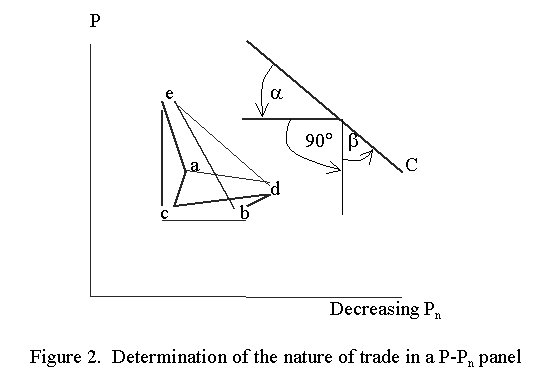
Examples of consistent trade are exports from e to a, from e to c, and from e to b, from a to c, and from d to c. There are two possible situations. When a + 90° < q < 180°, or q is bound by the vertical line and the iso-cost (or q falls in b), difference in P is more prominent than in P_n between the two positions (or two countries). A lower position at the southeast experiences a larger reduction in P than in P_n and thus P is reduced to a significantly smaller value than is P_n. Given C=P_n/P, this leads to a larger increase in C for the lower position. Secondly, when a < q < a +90°, a lower position at the southwest experiences opposite change in P and P_n, such as declining P and increasing P_n, and thus lowers both absolute and comparative advantage.

An opposing type trade occurs when absolute and comparative advantage principles point to opposite trade directions. For example, absolute advantage allows export from a to d, while comparative advantage allows an exactly opposite pattern. This is the most anti-intuitive aspect of the comparative advantage principle: countries with lower comparative cost have lower productivity, and export to more productive countries. An opposing trade occurs when 0 < q < a, and difference in P_n is more prominent than in P between two positions. A lower position at the southeast experiences a larger reduction in P_n than in P, leading to a fall in C at the lower position. A dichotomous type trade refers to the situation where trade is allowed by one principle but not by the other. For example, when q=0 (or the line connecting two points is parallel to iso-cost curves), absolute advantage principle allows export, such as from e to d, and a to b. However, comparative advantage principle does not allow such exports since two countries have the same comparative cost due to the same level of comparative cost between two points. When q=a (or the line connecting two points is parallel to the horizontal axis), comparative advantage principle allows trade, such as export from b to c, since P_n and, thus C differ between the two points. However, absolute advantage principle does not allow such trade since the two points have the same productivity.
 

Extension of the initial model.

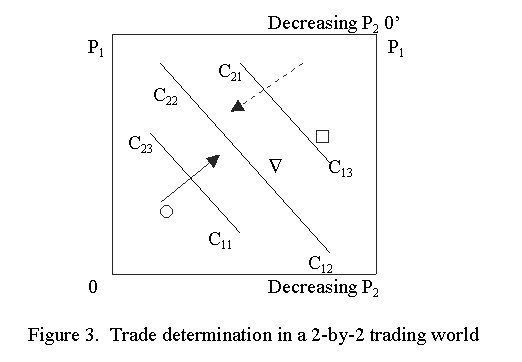
Figure 1 only illustrates comparative cost of one commodity using the second commodity as the numeraire. In a two-commodity trading world, commodities are used as the numeriare in turn. Figure 3 is constructed by drawing in two axes on the right and top sides in Figure 1. The axes labeled P₁ and P₂ denote productivity of the two commodities respectively. The left and bottom sides are used to determine the comparative cost of commodity 1 using commodity 2 as the numeraire. The solid arrow originating from corner 0 indicates declining comparative costs represented by C₁₁, C₁₂, C₁₃. The top and right sides are used to determine the comparative cost of commodity 2 using commodity 1 as the numeraire, and C₂₁, C₂₂, C₂₃ represent subsequently diminishing comparative cost from corner 0'. Since C₁=P₂/P₁=1/(P₁/P₂)=1/C₂, then C₁₁, C₁₂, C₁₃ and C₂₁, C₂₂, C₂₃ are the same set of iso-cost curves merely being reverse to each other. The dashed arrow originating from 0' gives the direction of declining comparative cost of commodity 2. It is immediately apparent that in a two-commodity trading world, if one country has comparative advantage in one commodity, it has comparative disadvantage in the second commodity. In Figure 3, the circle, triangle and square represent the positions of countries 1, 2 and 3 respectively. While Country 1 has comparative advantage in commodity 2, it has comparative disadvantage in commodity 1. The opposite can be said about Country 3. Country 2 is in an intermediate position. In terms of commodity 1, Country 2 has more comparative advantage than Country 1, but less than Country 3. For commodity 2, Country 2 has more comparative advantage than Country 3, but less than Country 1.
 

For a trading world with more than two commodities, a common numeraire can be chosen for all other commodities. The situation in Figure 3 can be repeated for more commodities, as shown in Figure 4. Four panels illustrate the comparative cost for commodities 1, 3, 4 and 5 using commodity 2 as common numeraire. As in Figure 3, Countries 1, 2 and 3 are represented by a circle, triangle and square, respectively. Horizontal axes in all panels denote decreasing productivity of commodity 2.
 

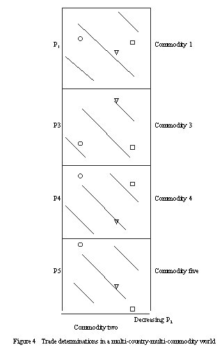
The comparative cost for different countries can be read for different commodities from Figure 4, and are shown in Table 1, and trade pattern based on comparative advantage can be deduced accordingly. The dark arrows in Figure 5 indicate the flow of commodities based on the low and high comparative cost in Table 1. For a country with medium comparative cost in a commodity, it may export or import that commodity depending on the actual quantity of supply and demand. A large demand from the import country and small supply from the export country will necessitate the export from the medium cost country. On the other hand, a large demand from the medium cost country itself may mean import.
 

Table 1 Comparative costs in a multi-country multi commodity world
 

	Commodity one	Commodity three	Commodity four	Commodity five
Country 1	High	High	Medium	Low
Country 2	Medium	Low	High	Medium
Country 3	Low	Medium	Low	High

 

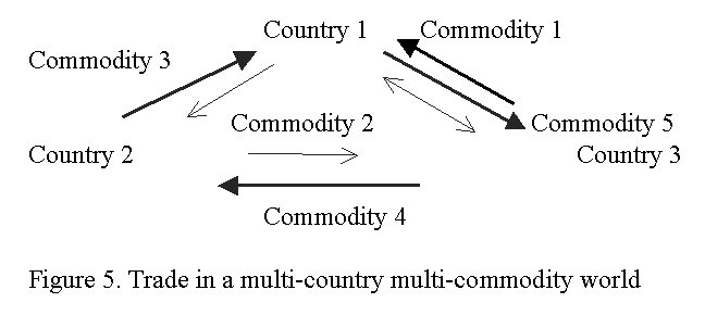
The overall pattern of comparative advantage in commodity 2, the numeraire, is not clear among the three countries. This is so since the comparative cost of the numeraire is expressed in different commodities in turn. It may be low in terms of one commodity but quite high in terms the other (Table 2). As a result, the trading pattern is circular, and one country exports as well as imports commodity 2 at the same time (light arrows in Figure 5). Commodity 2 provides counter flows to trade flows shown with dark arrows. It is clear that when a common numeraire is used to denominate other commodities, it serves as money in exchange. The important contribution of Ricardo's comparative advantage principle is the realization that productivity alone cannot determine trade. The introduction of the second dimension problematizes the pattern of those trades where 0 < q < a in Figure 2, and reveals the roles of the medium of exchange and unit of account in exchange.
 

Table 2 Comparative cost of commodity 2 expressed in different numeraire commodities
 

	In commodity 1	In commodity 3	In commodity 4	In commodity 5
Country 1	Low	Low	Medium	High
Country 2	Medium	High	Low	Medium
Country 3	High	Medium	High	Low

 

Neoclassical version of the model.

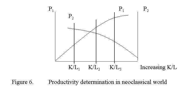
Haberler (1936) views the numeraire commodity as the opportunity lost in making the first commodity, and thus recast comparative advantage in a framework of opportunity cost. This is particularly appropriate for neoclassical trade theory, which attributes the cause of differing comparative cost to resource endowment and industrial resource use intensity, instead of labor productivity itself as in the classical trade theory. In other words, neoclassical theory advocates that resource endowment and industrial resource use intensity determine labor productivity, which in turn determines comparative cost. Heckscher and Ohlin's factor proportions theory states that a country has low opportunity cost or comparative advantage in a commodity if that commodity intensively uses an abundantly endowed resource in the country (Heckscher, 1935; Ohlin, 1933). To illustrate this point, use a neoclassical homogeneous production function Q=F(L, K) degree of one, where Q is the output, L and K are labor and capital inputs respectively. Dividing both sides of the function by L leads to P=f(K/L), where P is labor productivity and K/L is the capital-labor ratio. In Figure 6, the horizontal axis denotes resource endowment expressed by capital-labor ratio. Curve P₁ is the production function of a capital intensive commodity and curve P₂ the production function of a labor intensive commodity. Given three countries' resource endowment K/L₁, K/L₂, and K/L₃, their productivity in commodities 1 and 2 are determined by the intersections between the vertical lines and the production functions. Plotting the resultant productivity values on a panel like the one in Figure 3, the comparative cost and trade pattern can be determined, as done previously. For example, Country 1 has rich labor and scarce capital, which results in a lower P₁ but a higher P₂. This means a position at the circle in Figure 3, indicating a low comparative cost in labor intensive commodity 2. Country 3, on the other hand, has rich capital and scarce labor, and thus comparative advantage in capital intensive commodities. 1. Country 2 is in an intermediate position.

Recent developments.

The New Trade Theory (Krugman, 1981; Grossman and Helpman, 1989) in the 1980s is a methodological, instead of a conceptual, breakthrough in modeling trade. This is so because increasing returns to scale as a factor for trade has been recognized for a long time, along with factor endowments. What the new trade theorists break away from is the assumption of general equilibrium and associated perfectly competitive market in modeling trade. In the new framework, individual firms enjoying increasing returns to scale will grow in size and result in monopolistically competitively market structure. Differentiated commodities facilitate specialization and intra-industry trade. Leaving aside the mathematics and modeling tricks involved, the essential conclusion drawn by the New Trade Theory is quite simple: economies of scale improve productivity and therefore affect trade. In Figure 3, if P₁ increases as a result of economies of scale, the circle will move upward and comparative cost of commodity 1 will decrease. From previous analysis, other things being equal, an increase in productivity or an upward movement in the P₁-P₂ panel makes it more likely that a trade pattern is consistent with both absolute and comparative principles. After long period of effort in perfecting comparative advantage principles, the absolute advantage concept regained attention.

While the New Trade Theory mainly addresses the absolute advantage side of trade determination, the notion of competitive advantage proposed by Porter (2000) contains both comparative and absolute advantage elements with an emphasis on the latter. This notion situates actions of businesses and government amid a business environment consisting of supply conditions, demand conditions, and supporting industries. The three components in the business environment may arguably be approximated by a combination of endowment-based comparative advantage, demand preferences, increasing returns to scale, localization economies, urbanization economies, and even the roles of institutions. The driving forces in spatial exchange are the competitive behavior of firms and strategic actions of government. These dynamic aspects contrast with "static" endowment conditions in the traditional trade theory. Porter's narrow interpretation of the source of comparative advantage, as a result of factor endowment, helps highlight the role of dynamic actions of firms and government in shaping advantage in trade. The competitiveness as a result of strategic actions of businesses and government implies productivity and efficiency, which takes us back to Smith's absolute advantage principle. The debates on trade mechanism have gone full circle.

The changing emphasis on absolute and comparative advantage reflects the evolving intellectual interest in two fundamental sources of trade: productive efficiency and exchange efficiency. Productive efficiency expresses input-output relations and is influenced by labor force skills, quality of equipment, level of technology, increasing returns to scale, agglomeration economies, strategic actions of economic agents in technological and institutional innovations, etc. These factors are responsible for the vertical position of a commodity in a P-P panel. On the other hand, exchange efficiency reflects the output-output relations in commodity exchange. Differing from a production process, commodity exchange involves the use of a medium of exchange and unit of account. The consequence of using the numeraire commodity or money as the unit of account is that the (comparative) cost of a commodity varies vertically as well as horizontally on a P-P panel. Using a commodity, instead of an input, as a unit of account in exchange reflects the belief that the value of a unit of commodity is defined while that of a unit of an input is not. The value of a unit commodity lies within itself as a finished commodity, capable of satisfying a certain consumption need, no matter which country makes it. However, a unit of labor input is worth different amounts of a commodity (thus different value) if countries have different productivity. For example, in a P-P panel, the value of one labor hour measured in the numeraire varies along the horizontal axis. For a given P₁, an hour of labor input is worth more numeraire commodity when moving leftward along the P₂ axis. Since the comparative cost of a commodity is the units of the numeraire contained in a unit of that commodity, it is only natural that the commodity becomes more expensive (or contains more numeraire) when each hour of input is worth more of the numeraire commodity.

The comparative cost approach is a breakthrough in conceptualizing the unit of account in commodity exchange. In essence, it moved away from the labor numeraire toward a commodity numeraire. It is paradoxical that it is Ricardo who, as a classical economist adhering to the Value Theory of Labor, was the first to promulgate it. The commodity numeraire eventually becomes the conceptual underpinning in neoclassical general equilibrium analysis. This may explain the long lasting interest in the comparative advantage approach in trade determination. However, choosing a commodity numeraire only discredits the notion of socially necessary (or average) labor hours in value determination of a commodity. It does not eliminate specific productivity of a particular commodity from trade determination. One cannot talk about comparative advantage without differences in productivity as a basis. As shown above, the comparative cost is the ratio of numeraire productivity to productivity of a commodity. That comparative advantage is partly determined by productivity is underscored by Yang and NG (1993). They see the absolute advantage as a more general condition of trade since differences in productivity are the basis of comparative advantage. Grossman and Helpman (1989) recognize that New Trade Theory differs from the traditional trade theory in terms of sources of comparative advantage: the former is acquired while the latter is natural. The switching emphasis in recent trade study to absolute advantage may reflect a rising intellectual interest in more dynamic, fast changing, and real economic side in trade determination.
 

3. Recasting location theory from an exchange point of view

Trade theory provides a starting point from which to understand trade origin and trade pattern, mostly at the regional or national levels. We are also interested in knowing at what places export commodities are actually produced. This is the task of location theory. Although trade theory and location theory differ from a modeling technique point of view, as pointed out by Krugman (1993), there is profound conceptual overlapping between the two. The basic relationship is that location theory is a simplified and special case of trade theory. Neoclassical trade theory deals with location issues from an exchange point of view and addresses export and import simultaneously. It evaluates specialization at a location in conjunction with alternative industries and locations. On the other hand, location theory deals with location issues from either a production or demand point of view, and assesses a particular specialization among alternative locations. The main concern is to locate the production of an export commodity or service at a location. Imports of finished commodities are not explicitly addressed. These concerns help reduce the scope of, and simplify, trade theory. For example, in industrial location theory, the chief concern is the optimal location of export production and no attention is given to the importation of finished commodities. In agricultural location theory, the emphasis is to find locations for crops to be exported, rather than farmers' imports from a center city. In central place theory, the issue is to determine central places as locations for selling (exporting) services to customers within certain areas, instead of trade between different central places. However, location theory is also a special case of trade theory in that transport cost is an explicit consideration in location theory, which has largely been ignored in trade theory. In all of the above examples, transport cost plays a crucial role in shaping particular spatial configurations.

Even though the characteristics of location theory being a partial and special case of trade theory may not be entirely correctable (for convenience we may not even want to correct them), there are strong reasons for linking location theory to trade theory. The first is the role of locations in a regional or national economy. Although an export sector in location theory appears somehow "given" instead of being determined by comparison with alternatives, exchange is implicitly present and forms part of the discussion background. Absolute and comparative advantages do not exist equally on every location, and thus the degree of specialization is not uniform across a region or a country. Given a region's absolute or comparative advantage in a commodity, a location study helps pin down the optimal production site, or sites with strongest absolute or comparative advantage. From this viewpoint, location theory is a sort of follow-up study involving elements at a local scale after the general trade pattern is determined at a larger scale.

In addition, there is the issue of long-term balance of payment. A locational specialization is a symptom of export and import. Although one can assume that a location exports a commodity and relies on local supply for the rest of consumption, this situation cannot exist forever. A location with export but without import necessarily experiences trade surplus, and thus exports capital and accumulates financial assets. Exchange rates will come under pressure to rise. In addition, income growth as a result of export expansion leads to increased consumption and investment, further taxing the local resource base. Price and interest rates will eventually rise, reducing trade advantage and attracting capital inflow. A strong currency, rising prices, and high interest rates eventually will help reverse the trade pattern. The precondition for locational analysis of the export sector diminishes. Therefore, locations are a basis to achieve long-term macroeconomic equilibrium, and should be dealt with in a broader context.
 

Recasting central place theory.

Conceptually, an exchange framework can be explicitly used to recast location theory. Bogart (1998) places urban economy in a context of exchange and views metropolitan areas as a collection of small open economies trading with each other. Within a metropolitan area, different districts are seen as a collection of open economies that undergo commercial exchange. Such insightful observations have important implications for conceptualizing central place theory from a trade point of view. The traditional central place study bases the function of a place on its size and the threshold of economic functions. Places have different economic functions due to their sizes that meet demand threshold of various functions (Christaller, 1933; Lösch, 1940).

As in any division of labor, a general advantage in separating various functions or functional combinations among different centers is the improved productivity. This results from the ease in coordinating and reinforcing regulations and ordinances consistent with the function of a place, eliminating potential conflicting requirements, and thus lowering transaction cost. The pattern of division of labor can be examined using an exchange framework in which a central place system acts as a hierarchical-locational specialization-trading system. Larger centers "export" to surrounding smaller communities specialized commercial and industrial functions unique in large places. Smaller centers specialize in providing residential function and living environment. The basis of specialization and exchange is absolute and/or comparative advantage. Larger centers, due to their size, accessibility and centrality, provide a larger quantity of diverse resources more necessary for large businesses than smaller centers. Consequently, larger businesses, especially those experiencing increasing returns to scale, are more likely to be located in more centrally located larger centers to maintain high productivity. Smaller businesses are located both in larger and smaller centers due to their lower resource requirement. As a result, resource constraints, in addition to demand threshold as in the traditional central place study, are crucial factors that influence productivity of businesses, and thus their distribution among centers of different sizes.

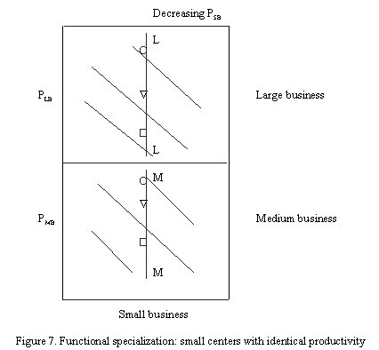
In the P-P panel in Figure 7, P_LB, P_MB, and P_SB denote productivity of large, medium, and small sized businesses, respectively. In the P_LB-P_SB panel, a large place, indicated by the circle, allows a high productivity in the large business; a small center, the square, allows a low productivity for the large business, and a medium sized center, the triangle, takes the middle ground. All places allow equal productivity for the small business. The result is that the large place has a low comparative cost for large businesses and the small place has a low comparative cost for small businesses. The medium sized place has lower comparative cost in large businesses than the small place, and has lower comparative cost in small businesses than the larger place. In the P_MB-P_SB panel, the large place still generates the highest productivity for the medium sized business. However, due to less resource constraints, the medium sized business has higher productivity in the medium and small-sized centers compared with that for large businesses, reflecting in the positions of the triangle and square in two panels.
 

The above analysis of three centers can be generalized to include all centers in an urban system. Vertical curves LL and MM are the result of connecting comparative costs of all places of different sizes from small (bottom) to large (top) in the two panels. Re-mapping LL and MM in Figure 8, it becomes apparent that comparative cost of large businesses is lowest only in large centers. In comparison, comparative cost of medium sized businesses are low both large and
 

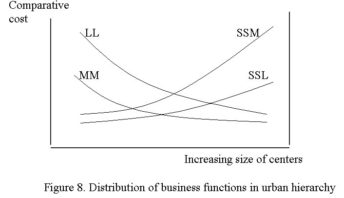
medium sized centers. In addition, in small centers, comparative cost for medium sized businesses is lower than for large businesses. SSL and SSM are comparative cost of small businesses using large businesses and medium sized businesses as the numeraire respectively. Although not directly comparable between SSL and SSM, it is clear that the cost of small businesses is the lowest in small centers. These conclusions suggest a pattern of hierarchical distribution of businesses, in which large businesses are overwhelmingly concentrated in large places, small places have predominately small businesses, and medium sized businesses are more likely located in small and medium sized places.

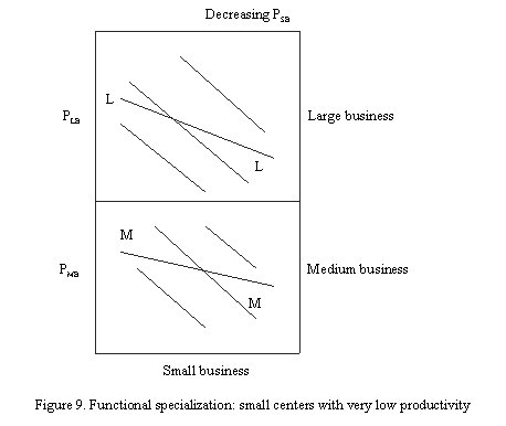
The above conclusions are partly influenced by the assumption that small businesses have the same productivity regardless of the size of places. In reality, agglomeration economies tend to increase with the size of places, which will benefit small and large businesses alike. Therefore, small places will be less productive than large places even for small businesses. 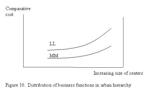Figure 9 shows a urban productive system where large businesses are more productive in large centers than in smaller centers, but small businesses are so unproductive in smaller centers that large businesses have a low comparative cost in smaller centers than in larger centers (Figure 10). For similar reasons, medium sized businesses could have lower comparative cost in smaller places than in large places. These point to the condition for the diffusion of large and medium sized businesses to smaller centers. This shows that low productivity of local commercial and manufacturing businesses in small centers, remote areas or developing countries may not necessarily be a constraint in their economic growth. In an open exchange economy, it is exactly the low productivity in these local businesses that leads to the low comparative cost that attracts investment from outside retail chains, national companies or multinational corporations.
 

Recasting agricultural location/land use theory.

In his path-breaking work, Alonso (1964) incorporates neoclassical substitutable technology into land use study and essentially transforms von Thünon's classical agricultural location theory (1826) into the factor proportions theory. Figure 11 portraits a typical pattern of land price/rent, denoted by r, and prices of other inputs such as wages denoted by w, from a city outward.
 

The steeper slope of the r curve than that of the w curve makes it plain that resource endowment varies from the one extreme of scarce land close to the city to the extreme of ample land at the horizon. The endowments in the intermediate positions change gradually from more land scarcity to less land scarcity. If a series of zones are drawn surrounding the city, different zones have different resource endowments suitable for farming/ land use systems of various resource use intensity. This is exactly the kind of situation where a neoclassical production shown in Figure 6 and neoclassical trade scheme fit in. 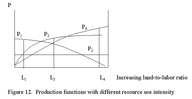Land further away from the city has lower opportunity cost (or comparative advantage) in land intensive activities, while land closer to the city has lower opportunity cost (or comparative advantage) in other input intensive activities. Figure 12 illustrates production functions of four industries with industry 1 being labor intensive, industry 4 land intensive, and industry 3 in a intermediate position. According to production theory, in areas richly endowed with labor, industry 1 has the highest productivity; in areas with abundant land, industry 4 shows the highest productivity. Industry 3 has the highest productivity in areas with intermediate land and labor endowment. Industry 2 has identical productivity in areas of different resource endowment, and is used as a numeraire. 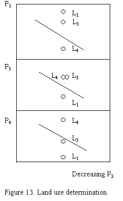Three representative locations L₁, L₃ and L₄ are shown in Figure 12, and mapped on Figure 13 in different farming/ land use system panels. It is apparent that the lowest comparative cost occurs at location 1 for industry 1, at locations 3 and 4 for industry 3, and at location 4 for industry 4. Land adjacent to these three locations form three farming/land use zones surrounding the city, specializing in industry 1, a mix of industries 3 and 4, and industry 4 respectively. If the numeraire commodity is considered, the specialization pattern should be a mix of industries 1 and 2 in a zone close to the city, a mix of industries 3 and 4 in the zone in the middle, and a mix of industries 2 and 4 in the zone furthest from the city.
 

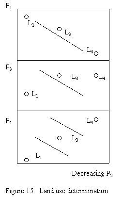
The above specialization pattern occurs partly due to the assumption of the identical productivity of industry 2 across all locations. Suppose industry 2 is labor intensive and thus its productivity declines with increasing labor scarcity, as shown in Figure 14. Mapping productivity of industries onto the P-P panel leads to Figure 15. It is clear that using a labor intensive industry as the numeraire reduces the comparative advantage of existing labor intensive industries and
 

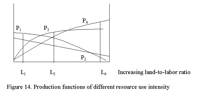
enhances comparative advantage of non-labor resource intensive industries. This highlights how the uneven distribution of the numeraire can alter the distribution of comparative advantage and thus the pattern of trade. Since money is the ultimate numeriare in a monetary exchange economy, this essentially points to the impacts of differential money supply and price level on geography of exchange.
 

Recasting industrial location theory.

There have been a numerous studies that incorporate neoclassical production theory into Weber's (1909) classical industrial location theory (Moses, 1958; Khalili, et al. 1974; Heaps, 1982; Shieh and Mai, 1984). An alternative approach is to incorporate trade theory into Weber's tradition. Suppose that there is a regional economy in the locational triangle region that is endowed with two inputs m₁ and m₂, and produce two commodities G₁ and G₂. Of the two commodities, G₁ is m₁ intensive while G₂ is m₂ intensive. As in a typical location triangle, as shown in Figure 16, inputs m₁ and m₂ are supplied from the two corners on the top and the export market of the regional economy is M. The issue is to find a most advantageous location for production. Suppose that in order to produce any commodity, the regional economy has to ship m₁ and m₂ to an ideal site. The annual productive capacities in m₁ and m₂ determine all the resources the regional economy can use. The dashed curve in Figure 17 indicates a G₁-G₂ production frontier as a result of the annual productive capacity of the two inputs.
 

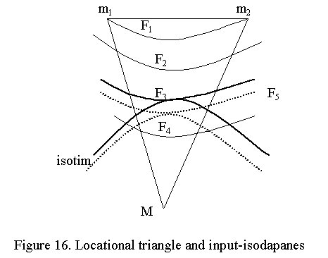
The actual amount of resources available at the location of production for producing G₁ and G₂ is less than the annual productive capacity since some inputs will be used to develop a transport sector for shipping inputs and the finished products. The arcs F₁, F₂, F₃, F₄, … in Figure 16 are lines with equal total input shipping cost, called the input-isodapanes. Suppose that the same proportion of m₁ and m₂ is used in the transport sector as that of the region's endowment of m₁ and m₂. In other words, the ratio of m₁ to m₂, which is used to build the transport sector, is the same as the m₁ to m₂ ratio for the region as a whole. This will cause a parallel downward shift of the production frontier in Figure 17. On different input isodapanes, there will be different amounts of inputs available to produce commodities, but the ratio of m₁ to m₂ is the same.

The above assumption means that if the region as a whole is endowed with rich m₁ and scarce m₂, so is the location of commodity production. According to the factor proportions principle, the opportunity cost of G₁ is lower and the region or the location of commodity of production will export G₁ to, and import G₂ from, M. The issue is to find the optimal location of commodity production.

A downward shift of the production frontier is caused by the cost of shipping inputs and cost of shipping G₁ to M. The optimal location occurs where the downward shift of the production frontier is a minimum. At such a location, for a given cost of shipping inputs (i.e. along a given isodapane), the lowest cost of shipping a given amount of finished commodity G₁ always occurs at a location closest to the market. This determines that the optimal location occurs at the tangent point between an arc and an isotim of G₁, the curve of equal shipping cost of the finished commodity. One such example is given in Figure 16 as the tangent between F₃ and an isotim. This optimal location is found through such a process. Along F₁ there is a slight downward shift of the production frontier due to short distance and thus smaller input shipping cost, but a significant downward shift due to long distance and thus larger cost of shipping a given amount of G₁ to market M. The net result is a significant downward shift of the production frontier to T₁ in Figure 17. On the other hand, along F₄, there is a significant downward shift of the production frontier due to long distance and thus a larger cost of shipping inputs, but a slight downward shift due to short distance and thus smaller shipping cost of the given amount of G₁. The net position of the production frontier is at T₄ in Figure 17. In general, for a given amount of export of G₁, from F₁ to F₂ to F₃ to F₄, the downward shift due to the cost of shipping inputs increases, and downward shift due to the cost of shipping final product decreases. The optimal location occurs where the marginal downward shift due to shipping inputs equals the marginal downward shift due to shipping the output. At this point, the combination of downward shift of the production frontier from both costs is a minimum. Therefore, T₃ in Figure 17 gives the highest position of the production frontier along F₃ at the tangent point with the isotim in Figure 16.
 

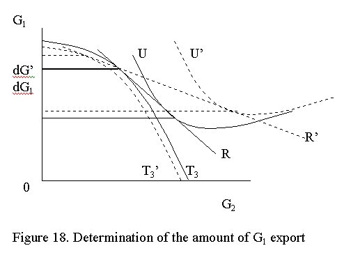
The conclusion reached so far is similar to Weber's original work, though it is now based on a regional exchange model. A particular advantage of such an exchange framework is its general equilibrium setting. For example, when terms of trade change due to supply or demand conditions, the amount of export of G₁ will change, which in turn affects the optimal location. In Figure 18, U is a particular utility level in the region's utility function. Straight line R is the term

of trade between G₁ and G₂. The difference between two horizontal lines, dG₁, indicates the amount of export of G₁ to M. When R changes, dG₁ changes. This causes the total shipping cost of G₁ to change, and thus the optimization process described above to readjust at the new level of G₁ export. In Figure 18, a new terms of trade, dashed line R', changes export of G₁ to dG' indicated by the gap between two dashed horizontal lines. Via readjustment process, a different minimum downward shift of the production frontier establishes, indicated by the dashed production frontier T₃'. A different pair of isodapane and isotim will produce a tangent point as the optimal location of commodity production, as the dashed input-isodapane and dashed isotim show in Figure 16.
 

One can go one step further to incorporate the notion of hierarchy into the industrial location analysis. For example, assume that G₁ production is subject to increasing returns to scale. Such a condition requires G₁ be located at a larger center where there is lower opportunity cost for large businesses as stated above. The production frontier will shift downward more when the production site moves away from the tangent point between an input isodapane and an isotim. However, increasing returns to scale will cause an upward shift of the production frontier. As long as the upward shift is more than the downward shift, the larger center is justified as the production site. Again, the conclusion is somewhat similar to Weber's original discussion of the impacts of agglomeration economies in selecting a location. The process of determining the site of an economic activity involves locating a hierarchical position and a geographical location simultaneously.
 

3. Summary and concluding remarks

This paper sets out to address a few shortcomings in current trade study within economic geography. The trade model developed in the paper allows one to dissect the roles of commodity productivity and the numeriare in determining absolute and comparative advantage. Also, the model is reasonably general to extend to multi-region and multi-commodity trades. In addition, the model provides a framework to reveal underlying causes of consistent, opposing, and dichotomy trades. The significance of such a model is that it is flexible enough to express essence of classical trade theory, neoclassical theory, New Trade theory, and competitive advantage theory in a unified framework. In addition, the model makes it easy to incorporate the impacts of money into trade analysis.

Using the trade model, the paper recasts location theory in an exchange framework. In such exchange framework, central places are shown to specialize in particular functions as a result of absolute and comparative advantage associated with the size of businesses and resource constraints of places of different sizes. Allocation of agricultural system/land use surrounding a city is achieved as a result of resource endowments and industrial resource use intensity. In addition, the classical industrial location model is placed in a regional exchange economy, and the optimal location is found to be the location of actual exchange between export and import. Recasting location theory in an exchange framework allows an in-depth understanding of a location's significance from a broader context. It provides a consistent conceptual basis for the follow-up investigation to supplement the traditional trade study. Trade theory provides a unified framework for spatial analysis, with absolute/comparative advantage principle as underlying mechanism. Location theory can be treated as a special case of the more general theory of spatial specialization and exchange. Since trade theory and location theory can be essentially expressed as the same theory, the recent attention to trade theory and the marginalization of location theory are not justified.
 
 
 

Literature cited

Alonso, W. 1964. Location and Land Use: toward a General Theory of Land Rent. Cambridge, Harvard University Press.

Bogart, W.T. 1998. The Economics of Cities and Suburbs. Upper Saddle River, NJ, Prentice- Hall, Inc.

Christaller, W. 1933. Central Places in Southern Germany. English translation: Englewood Cliffs, N.J., Prentice-Hall, 1966.

Grossman, G. and Helpman, E. 1989. Product development and international trade. Journal of Political Economy (97), 1261-83.

Haberler, G. 1936. The Theory of International Trade. London: W.Hodge & Co.

Heaps, T. Location and the comparative statics of the theory of production. Journal of Economic Theory (28): 102-12.

Heckscher, E. F. 1935. Mercantilism. London: Allen & Unwin.

Khalili, A., Mathur, V.K. and Bodenhorn, D. 1974. Location and the theory of production: a generalization. Journal of Economic Theory (9): 467-75.

Krugman, P. R. 1993. On the relationship between trade theory and location theory. Review of International Economics (1): 110-122.

______. 1981. Intra-industry specialization and the gains from trade. Journal of Political Economy (89): 959-73.

Lösch, A. 1940. The Economics of Location. English translation: New Haven: Yale University Press, 1954.

Moses, L. N. 1958. Location and the theory of production. Quarterly Journal of Economics (72): 259-72.

Ohlin, B. G. 1933. Interregional and Interregional Trade. Cambridge, Harvard University Press

Porter, M. E. 2000. Locations clusters, and company strategy. In G.L. Clark et al. (ed) Oxford Handbook of Economic Geography. Oxford, Oxford University Press.

Ricardo, D. 1817. The Principle of Political Economy and Taxation. London: Gaernsey Press, 1973.

Shieh, Y. and Mai, C. 1984. Location and the theory of production: clarifications and extensions. Regional Science and Urban Economics (14): 199-218.

Smith, A. 1776. An Inquiry into the Nature and Causes of the Wealth of Nations. Chicago: University of Chicago Press, 1976.

Weber, A. 1909. Theory of the Location of Industries. English translation: Chicago: University of Chicago Press, 1958.

Yang, X and NG, Y-K. 1993. Specialization and Economic Organization: a New Classical Microeconomic Framework. New York, North-Holland.